Atmospheric Aircraft Modeling and Design
This section includes several examples of atmospheric vehicle modeling using the Flixan flight vehicle modeling program to create state-space systems for control analysis and simulations. The models include structural flexibility, propellant sloshing, and tail-wags-dog dynamics which interact with the aerosurface actuators or TVC. Several types of actuator examples are included, which are generated by the Flixan actuator modeling program.
The examples include the Space Shuttle during reentry, missile designs, fighter aircraft, reentry glider designs from space to landing, hypersonic rocket planes and 6DoF simulations implemented in Simulink. The controllers are designed using the Flixan program and analyzed both in Flixan and Matlab.
Space Shuttle During Hypersonic Reentry
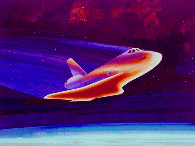
In this example we will analyze the Space Shuttle Orbiter and design a flight control system during early atmospheric entry from space where the dynamic pressure is low, the vehicle speed is hypersonic, and the angle of attack is high for speed-breaking. Prior to reentry the vehicle ignites the orbital maneuvering engines to reduce its orbital speed to allow gravity to take effect and it maneuvers using the RCS jets and enters the atmosphere with a shallow flight path angle and at 40° angle of attack. The vehicle also banks at 80° to ensure atmospheric penetration and avoid bouncing back into space. Precise angle of attack control is important during early entry because (a) regulates the heat dissipation caused by atmospheric friction. The angle of attack also controls the flight path angle g which is initially shallow, less than -1° to avoid overheating. The guidance system uses a preselected alpha reference as a function of velocity to manage temperature and to assure a safe heat dissipation rate. Excess kinetic energy is dissipated by roll maneuvers (S-turns) to control the down-range and cross-range position. During roll maneuvering the orbiter rolls about the velocity vector V0 to minimize the beta angle and side loads. As the vehicle descents to lower altitudes the angle of attack is reduced by adjusting the positions of the elevons and body-flap and the vehicle switches to normal acceleration (Nz) control. After a period of about 30 minutes from reentry the vehicle glides down unpowered and lands on a runway.
Design of a Missile with Wings
In this example we will analyze a cruising missile that has a small wing to provide lift and a fixed thrust engine that neither gimbals nor throttles. The missile is released horizontally from an aircraft and it climbs at high altitudes. It is controlled by three rotating aerosurfaces located in the tail section consisting of a vertical rudder mainly for yaw control, and two horizontal fins for pitch and roll control. There are no control surfaces on the wing. Since the engine is not gimbaling, it is the wing in combination with the elevon aerosurfaces that provides the necessary lift for the vehicle to climb. The attitude, rate, and acceleration are measured by an IMU located in the front section. The angles of attack and sideslip are not measured relative to the wind but the flight path angle g and the heading direction x are estimated inertially from navigation. We will use the Flixan program to generate dynamic models at a critical flight condition, which is: Mach 2.5, 10 degrees of angle of attack, and at high dynamic pressure of 1220 psf. We will design control laws for the pitch and lateral dynamics and analyze the vehicle stability and performance. I
F16 Fighter Aircraft Control Design and Simulation
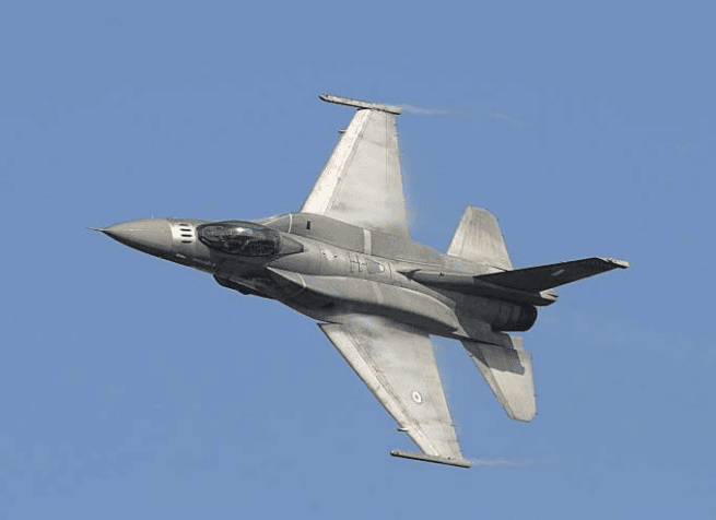
In this example we will use the Trim program to analyze stability and performance of the F-16 aircraft in different flight conditions along a couple of trajectories from take-off to landing. The aircraft has a single engine with a thrust that can vary from zero to 28,000 (lb). It is controlled by three aero-surfaces: an Elevon, an Aileron and a Rudder. The aerodynamic and mass-properties data were obtained from Brian L. Stevens and Frank L. Lewis book “Aircraft Control and Simulation”. The trajectories perform several types of maneuvers at different speeds, angles of attack, and bank angles. We will use the Trim program to analyze the vehicle performance, trim-ability, stability, and maneuverability along two trajectories. We will use the Flixan vehicle modeling program to create dynamic models at different flight conditions and use them for flight control design and analysis. We will also design state-feedback control laws for a range of angles of attack and dynamic pressures. We will finally create a 6DoF non-linear simulation in Matlab/ Simulink that uses the control laws by interpolating the gains as a function of alpha and dynamic pressure.
Design and Analysis of a Reentry Glider Vehicle
In this example we will use the Flixan/ Trim program to analyze the performance of a reentry, Shuttle type of unpowered vehicle in different phases during descent from early reentry to landing. Descent begins after firing the orbital maneuvering engines to slow-down, pitch attitude maneuver to position itself at an angle of attack of approximately 40°, and gravity begins to reduce its altitude and flight-path angle to g=-1°. Initially the dynamic pressure is very low and the vehicle uses reaction control jets for attitude control. Later it uses RCS in combination with aero-surfaces for trimming and control. As the dynamic pressure increases the aerosurfaces become more effective in controlling the vehicle and the RCS usage is reduced. The vehicle uses six aero-surfaces for trimming and control: 2 flaps, 2 rudders, a body-flap, and a speed-brake. The speed-brake is only used near landing for speed control. The body-flap is only used for trimming and not for flight control. Initially it is positioned at -20° which causes the vehicle to enter the atmosphere at a stable trim angle of attack a=40°. Although alpha is constant during the early part of reentry, the bank angle varies as the vehicle manages the excess kinetic energy. When the speed drops below Mach 1 the control mode switches to Nz-control, for controlling altitude, and the flight path angle comes down steeper at -20° to maintain high speed for the approach and landing maneuver. During the final flare maneuver the vehicle also uses its speed-brake for velocity control.
Autonomous Landing of a Glider Vehicle with Sloshing Tanks
In this example we will create longitudinal and lateral dynamic models of an un-powered Shuttle type of reentry glider vehicle that descends from high altitude and lands on a runway using an autonomous landing guidance system. The vehicle uses Elevon and Speed-Brake for longitudinal control, and Aileron and Rudder for lateral control. The dynamic models are further complicated by the sloshing of the residual RCS propellant inside the tanks that compromise the vehicle stability. The models are combined with the flight control and guidance systems, and used to analyze system stability in both pitch and lateral axes and to simulate the vehicle landing on a runway.
Actuator Examples
The following actuator modeling examples illustrate how to use the Flixan actuator modeling program to create 5 different types of actuator models ranging from simple generic, to electro-mechanical or hydraulic models using actuator parameters. The input data are located in file “Actor-Models.Inp” containing actuator data for the five modeling types. There is a batch set at the top of the file that can be used to process the entire file. The state-space systems are saved in file “Actor_Models.Qdr”.
Rocket Plane Control During Hypersonic Reentry
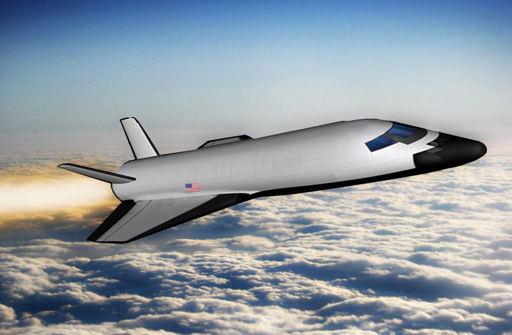
In this example we have a rocket-plane during level flight. It is controlled by five aerosurfaces and a fixed engine. The aerosurfaces are: two horizontal flaps, two rudders in a V-tail form and a body-flap in the back mainly for trimming. The engine is fixed and it does not gimbal and its thrust varies up to 4,000 (lbf) for acceleration and speed control. The control system controls altitude and airspeed in the longitudinal axes and in the lateral axes it controls the flight direction by means of roll control. We will analyze a single flight condition, at Mach 0.85, altitude 45,000 (ft), and dynamic pressure of 150 (psf). The analysis begins by creating dynamic models of the vehicle in this flight condition, design and analyze pitch and lateral control systems, introduce structural flexibility, aero-elasticity, and then evaluated the overall vehicle system stability and performance in response to commands and wind-gusts.
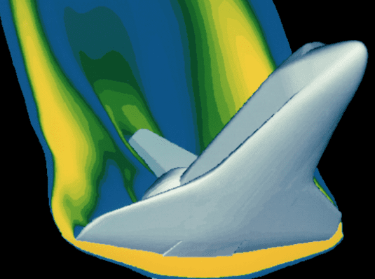
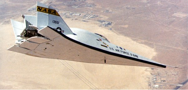
Lifting-Body Space-Plane Design and 6DOF Simulation
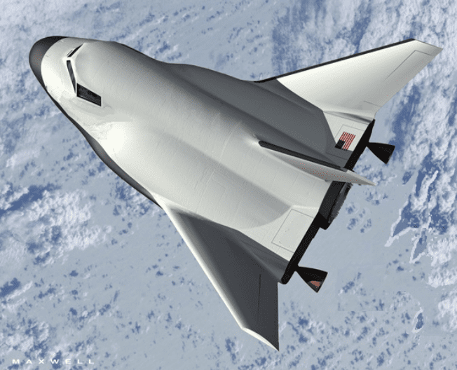
In this example we will analyze a Lifting-Body aircraft that is used as a space transportation vehicle, returning from space by gliding and landing autonomously by using its aerosurfaces. It is also capable of taking-off vertically like a rocket by means of two TVC engines, reaching high altitudes and then landing unpowered and autonomously. We will use the Flixan program to model and analyze this vehicle during both ascent and descent phases, demonstrate the entire flight control design from de-orbit to landing, beginning with a static performance and controllability analysis, control law design at selected Mach points, and linear dynamic analysis and simulation. This example teaches how to create linear dynamic models for flight control analysis, how to design simple control laws and how to create models for analyzing robustness to parameter variations. We also include a 6-dof non-linear reentry simulation from deorbit to landing created in Matlab/ Simulink. The second part of this example demonstrates the ascent phase when the two main rockets are firing.
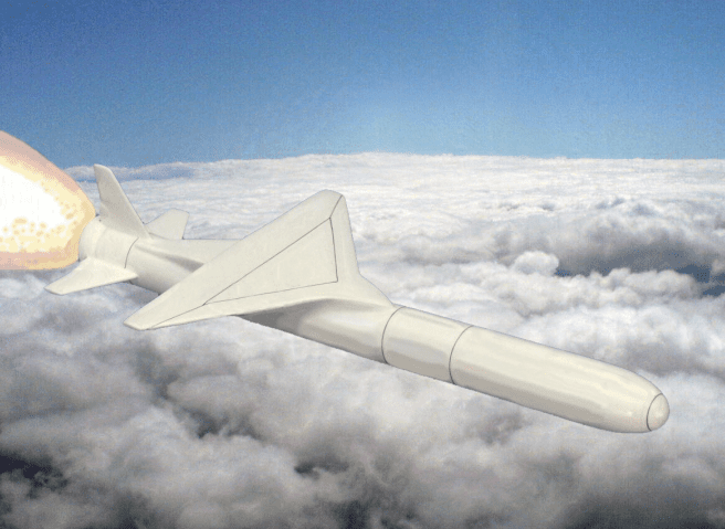
Hypersonic Rocket Plane Design
This example analyzes a rocket-plane that can either take off horizontally from the ground or it can be dropped from another aircraft. When it takes off from the ground it climbs up to an altitude of 76,000 feet. Then it turns off its engine and glides back to the ground and lands like an airplane using only aero-surfaces for control. The vehicle is powered by a 63,000 (lb) rocket engine during ascent and uses four aerosurfaces during both ascent and descent: an elevon, a body-flap, an aileron, and a rudder. We will use the “Trim” program to calculate the aero-surface trim angles and analyze the vehicle performance during the entire flight, from ground take off to landing. The analysis is separated into two parts, the boost phase and the descent to the ground phase. During ascent the rocket plane is controlled by the aerosurfaces and it uses a variable thrust fixed engine to regulate its axial acceleration. We will use the Trim program to calculate the trim angles of the control surfaces and the required engine thrust along the trajectory, analyze the vehicle static performance, investigate the effects of XCG variations on the effector trim angles and performance, analyze stability along the trajectory by using contour plots, and maneuverability against disturbances by vector diagrams. We will also take advantage of the multiplicity of pitch effectors to perform trim adjustments, and analyze the lateral axis effects of a beta disturbance and of YCG shifts.
Two Engine Supersonic Fighter Aircraft with Flexibility
In this example we will design the control system and analyze stability and performance of a supersonic fighter aircraft at a flight condition of: 20,000 (feet) altitude, level flight, at Mach: 1.4. The aircraft uses three aerosurfaces in combination with two thrust vectoring engines for flight control. The aerosurfaces are: two elevons (left and right) mainly for pitch and roll control, and a vertical rudder for yaw control. The two engines are gimbaling only in pitch to enhance pitch controllability and they can also vary their thrust for speed control. The nominal thrust of each engine in this flight condition is 30,000 (lb), but they can throttle above and below this thrust, from a minimum of 10,000 (lb) to a maximum of 50,000 (lb). The aircraft uses a vane sensor for measuring speed and the angles of attack and sideslip. Gyros are used for measuring body rates, and an IMU for attitude. Structural flexibility is also included in the finite element dynamic model. Inertial flex coupling coefficients are used to couple the effector motion with flexibility. The control objectives in this flight condition are to independently command and execute changes in altitude and velocity in the longitudinal directions and to control the bank angle in the lateral directions. The altitude and velocity are controlled by pitching and throttling the engines. The flight direction is controlled by rolling. A state-feedback control law is designed using the LQR method consisting of three loops that control: altitude, velocity, and roll attitude. The control system is also designed to tolerate a certain amount of wind gust disturbances.